A robot learns to climb a step

Lab 1 of 10 in Physical AI — ten labs that build one argument.

next: Biped Stairs →

Reading this without a background in machine learning

The plain words boxes like this one carry the whole story; the technical detail around them is there if you want it.

The one line version: we taught a one-legged robot to hop over a box, and found that paying it a bonus for being past the box rather than for crossing it made the best strategy to climb on top and stand there.

The first lab in 07_physical_ai, and the first in this course where the model acts on a world rather than on tokens. A three-link hopper stands in a 3D MuJoCo environment. Ahead of it is a box. The box is a different height every episode. It has to get past.

Everything is real: real contact physics, PPO written out rather than imported, real training on measured hardware. Nothing is pretrained and nothing is downloaded — the world is sixty lines of XML inside the source file.

The headline result is that the experiment this lab was designed around failed, and that turned out to be the most useful thing in it.

How this lab works

A one-legged hopper, a box on the floor, and a reward that pays for crossing it. The lab is about how easy it is to write a reward that pays for the wrong thing.

Same physics, same algorithm, same budget. The only change is whether the crossing bonus repeats — and with a repeating bonus the optimal policy is to climb on top of the obstacle and stay there, which scores beautifully and is not the task. Every later lab in this topic inherits the one-off rule.

The world

In plain words

A one-legged hopping robot, a flat floor, and a box in the way. It gets a reward for getting past the box.

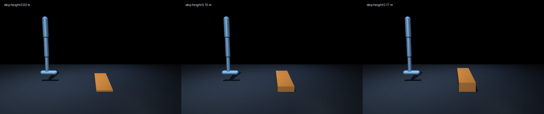
That is the actual simulation, rendered from the actual model — a floor, an orange step, and a three-link hopper: torso, thigh, shin, foot. The three panels are the same world at three draws of the obstacle height. On the left a 0.03 m lip you could stroll over; on the right a 0.17 m step that has to be climbed.

It is not a humanoid, and it does not walk on two legs. It has one leg and the torso is locked upright — with a free torso rotation this becomes the bipedal-balance problem, which is a famously hard benchmark and not what the lab is teaching. So it hops and lunges. Freeing that joint is the obvious next lab.

The two highlighted boxes are the premise. The obstacle height varies, and the policy can see it. A fixed obstacle would teach one gait; a range should force the robot to look and adapt.

Should.

The falsifier, stated first

If a policy that cannot see the obstacle height performs as well as one that can, then height perception is not what solves this task, and the headline claim of this lab is wrong.

--blind-to-height zeroes exactly that one input and changes nothing else. It is the same construction as test_omni_eval, which builds a model that ignores a modality on purpose and requires the harness to catch it. A claim that a robot "sees" something is worth nothing until blinding it costs something.

Training works

Baseline: a random policy, measured before every run — return 129, and it never even reaches the step. Budget: 600,000 environment steps, three seeds per arm, ~8 minutes each on CPU.

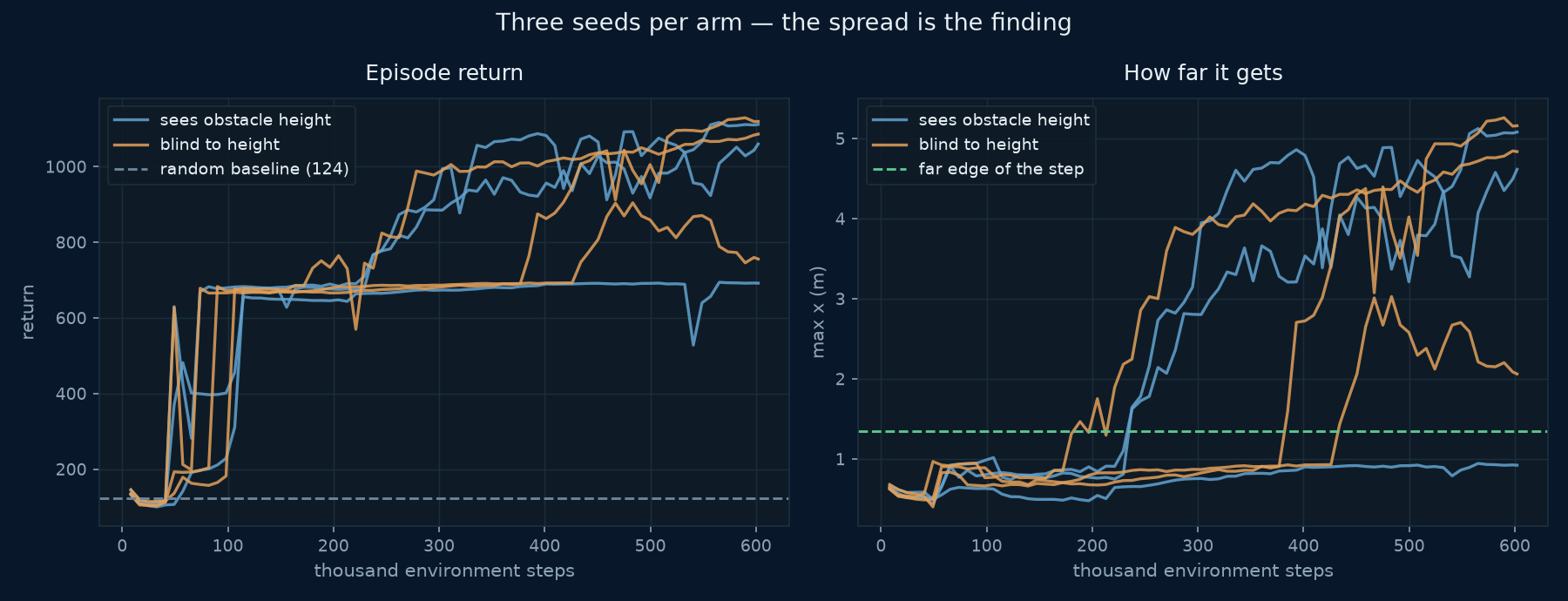
Both arms climb from 129 to roughly 1,000 — about 7× the baseline. The shape matters more than the number. There is a long plateau near return 670 where the robot has learned to stand and shuffle without going anywhere, then an abrupt breakthrough into real locomotion.

Every seed breaks through at a different time — 200k, 230k, 380k, 430k steps — and one seeing seed never breaks through at all. That flat blue line at the bottom of the right-hand panel is a run that trained for 600,000 steps and learned to stand still.

What training looks like

Same obstacle, same seed, same starting state. The only difference between these two clips is 600,000 steps of PPO. The panel is read from the live simulation every frame — nothing in it is pre-baked.

Before training — the random policy

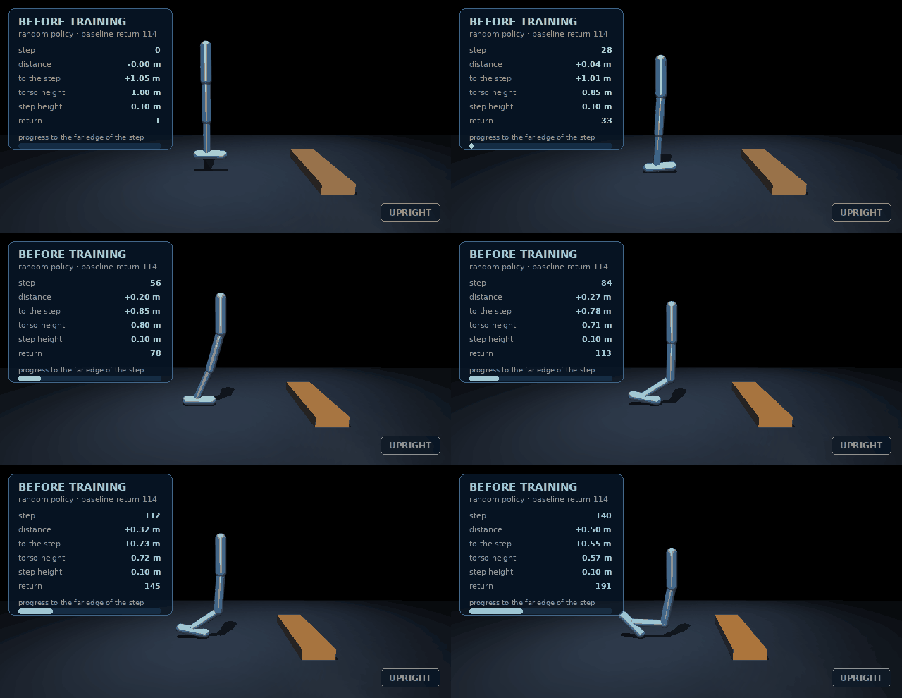
It topples almost immediately. Watch torso height fall from 0.99 m and the status flip to FALLEN when it crosses 0.55 m, which is the termination condition. distance never passes about 0.2 m, so the robot does not come close to the step at 1.05 m, and the progress bar barely leaves the left edge.

This is not a hand-picked bad run. It is the random policy — the measured baseline every number on this page is quoted against, return ≈ 114 against the trained policy's ≈ 1112.

After training — 600k steps of PPO

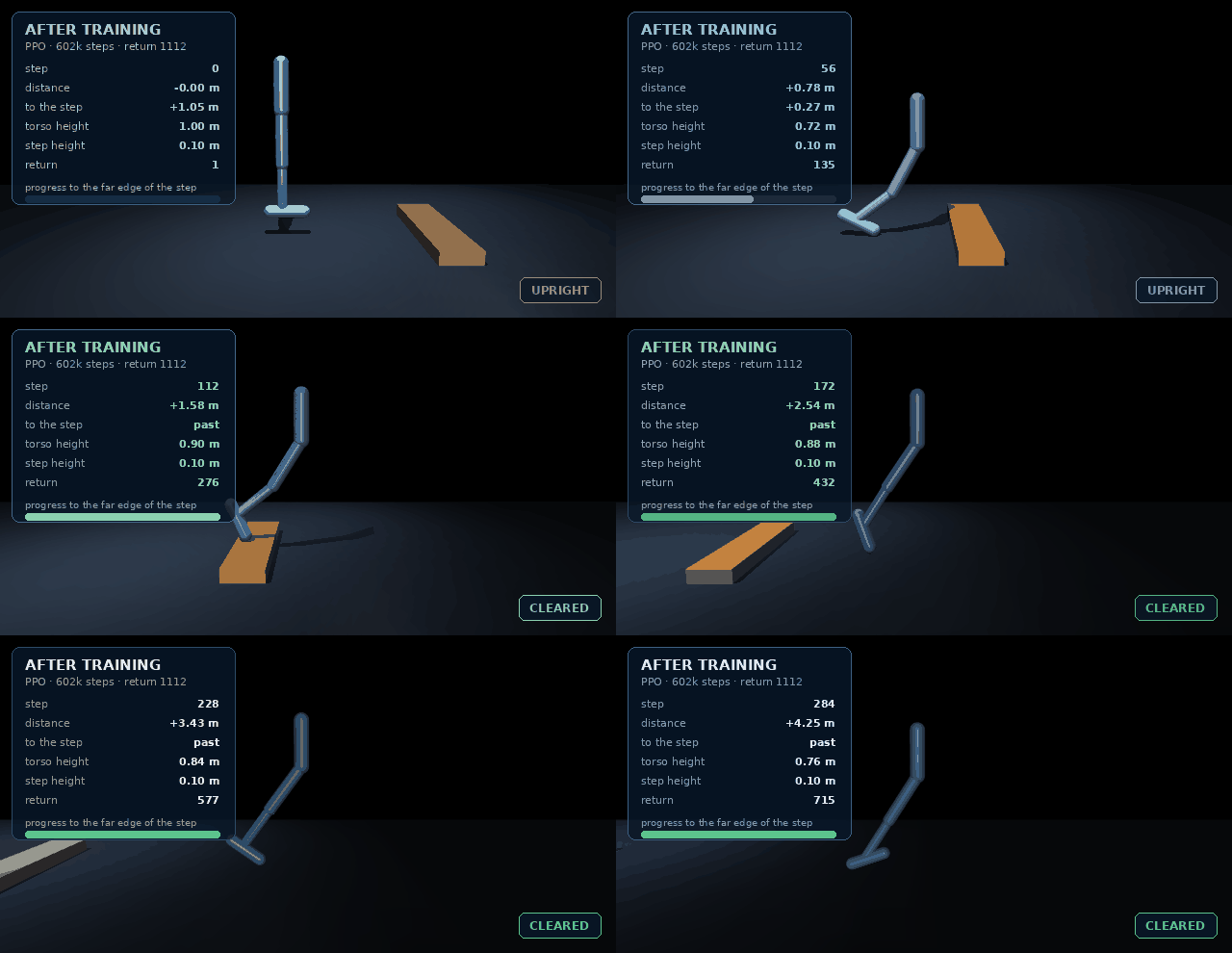
It drives forward, gets over the step, and keeps going. Three things in the panel are worth watching together: to the step counts down and then reads past; the status chip turns CLEARED; and return climbs steadily instead of flatlining, because the alive bonus keeps paying while the robot stays up.

The orange box scrolling off to the left is the camera tracking the robot — the step moving behind it is the robot clearing it.

Be precise about what this is and is not. The gait is a forward lunge, not smooth walking: one leg and a locked torso leave no other option. And on a 0.15 m step it gets past and then stalls rather than striding away — the sweep further down shows exactly where that limit sits.

Build one yourself

If you write software but have never touched reinforcement learning, this is the part to read. There is less to it than the vocabulary suggests, and nothing below is pseudocode — it is the lab, quoted.

An environment is a class with two methods

That is genuinely the whole interface. If you have written a state machine or a game loop, you already know this shape:

obs, info = env.reset(seed=0)            # start an episode
obs, reward, terminated, truncated, info = env.step(action)

• observation — what the agent is allowed to see this tick. An array of floats. Here, 11 of them.
• action — what it is allowed to do. Also an array of floats. Here, 3 joint torques in [-1, 1].
• reward — one number per tick saying how that went. This is the only channel through which you express what you want.
• terminated — it failed (the robot fell). truncated — it ran out of time. They are separate because the first is the agent's fault and the second is not.

A policy is just a function obs -> action. Training is the process of improving that function. Everything else is machinery.

The world is a scene graph, written in XML

This is the part people assume is hard. It is a tree of bodies, each with a shape and a joint, and MuJoCo does the physics. The entire world in this lab, trimmed to its skeleton:

<mujoco model="obstacle_hopper">
  <option integrator="RK4" timestep="0.002"/>
  <worldbody>
    <geom name="floor" type="plane" size="40 2 0.1"/>
    <geom name="step"  type="box" pos="1.2 0 0.05" size="0.15 0.6 0.05"/>

    <body name="torso" pos="0 0 1.0">
      <joint name="rootx" type="slide" axis="1 0 0"/>   <!-- move forward -->
      <joint name="rootz" type="slide" axis="0 0 1"/>   <!-- move up      -->
      <geom type="capsule" fromto="0 0 0 0 0 0.35" size="0.06"/>

      <body name="thigh">
        <joint name="thigh_joint" type="hinge" axis="0 -1 0" range="-150 0"/>
        <geom type="capsule" fromto="0 0 0 0 0 -0.42" size="0.05"/>
        <!-- shin and foot nest the same way -->
      </body>
    </body>
  </worldbody>

  <actuator>
    <motor joint="thigh_joint" ctrlrange="-1 1" gear="150"/>
  </actuator>
</mujoco>

Four concepts and you can build any world you like:

tag	what it is
geom	a shape that collides. plane, box, capsule, sphere, mesh
body	a frame that moves. Nest them and you have a kinematic chain
joint	how a body may move relative to its parent. hinge rotates, slide translates
actuator	a motor the policy can command. One entry per controllable joint

There is no rooty hinge in this model, and that omission is the single most consequential line in the file. Add it and the torso can rotate; the robot now has to learn balance before it can learn anything about obstacles, and 1M steps of training produced something that dived forward and fell over at one second.

The reward is four lines

forward = (x_after - x_before) / self.dt

reward = forward + 1.0 - 1e-3 * float(np.sum(np.square(action)))
if self.cleared() and not self._cleared_awarded:
    reward += 5.0                      # once, on clearing
    self._cleared_awarded = True

Read it as four separate instructions: go forward, stay alive (the +1.0 every surviving tick), do not flail (a small penalty on torque), and a bonus for getting past the box.

The +1.0 is doing more work than it looks. Without it the policy learns to fall over immediately, because falling ends the episode and ends the accumulating control cost. Reward design is mostly this: noticing which degenerate strategy you have accidentally made optimal.

The one-off bonus must be one-off. Pay it every tick and standing on the box forever beats crossing it.

What the policy sees

return np.concatenate([
    q[1:],                        # torso height + 3 joint angles   (4)
    np.clip(v, -10.0, 10.0),      # 5 velocities                    (5)
    [BOX_FRONT_X - q[0]],         # distance to the box             (1)
    [height],                     # how tall the box is this episode(1)
]).astype(np.float64)

Note what is excluded: the absolute x position, q[0]. Plain locomotion is translation-invariant — a gait is the same wherever you are — so feeding the world coordinate invites the policy to memorise a position instead of learning a behaviour. The relative distance to the box is the useful form of the same information.

Velocities are clipped because an early, bad policy can produce enormous ones, and a single outlier observation will wreck the running normaliser that everything downstream depends on.

The loop, in outline

for iteration in range(...):
    # 1. collect: run the current policy for N steps across 16 envs
    # 2. score:   compute_gae(rewards, values, dones, ...) -> advantages
    # 3. improve: a few epochs of clipped_policy_loss on that batch

That is PPO. Step 2 asks was that action better or worse than expected? and step 3 nudges the policy toward the better ones — but only within a trust region, so a single strange batch cannot destroy a working policy. Both are a dozen lines each in ppo.py, and both are exactly testable without a simulator.

Things to change first

In rough order of how much you learn per minute spent:

1. BOX_HEIGHT_MAX — push it past 0.17 and watch the clear rate collapse. This is the fastest way to see a task become unlearnable.
2. The reward. Delete the +1.0 alive bonus and watch the policy discover that falling over immediately is optimal.
3. A second box, further along — one more <geom> line.
4. Un-comment the rooty joint. The robot can now tip over. This is a genuinely hard problem; budget millions of steps, and expect it to need reward shaping you have not thought of yet.
5. Swap the robot. Gymnasium ships standard MuJoCo models (Ant, Half-Cheetah, Walker2d) whose XML you can drop in and point this same training loop at.

What will go wrong

Not might — will. These cost hours each while building this lab:

• It trains to something, and the something is nothing. Always measure a random baseline first and keep it on the chart. train_ppo.py runs 20 random episodes before every training run for exactly this reason.
• Your obstacle does nothing. This lab shipped a 100% clear rate against a box the robot was never touching. Test the physics directly, not through a policy.
• Normalisation. Observations mixing radians near zero with velocities in the tens will not train. If a correct-looking PPO learns nothing at all, suspect this before suspecting the algorithm.
• One run means nothing. See the entire next section.

The result: the ablation failed

arm	seed 0	seed 1	seed 2	mean
sees height	1060	1112	692	955
blind to height	1119	1086	756	987

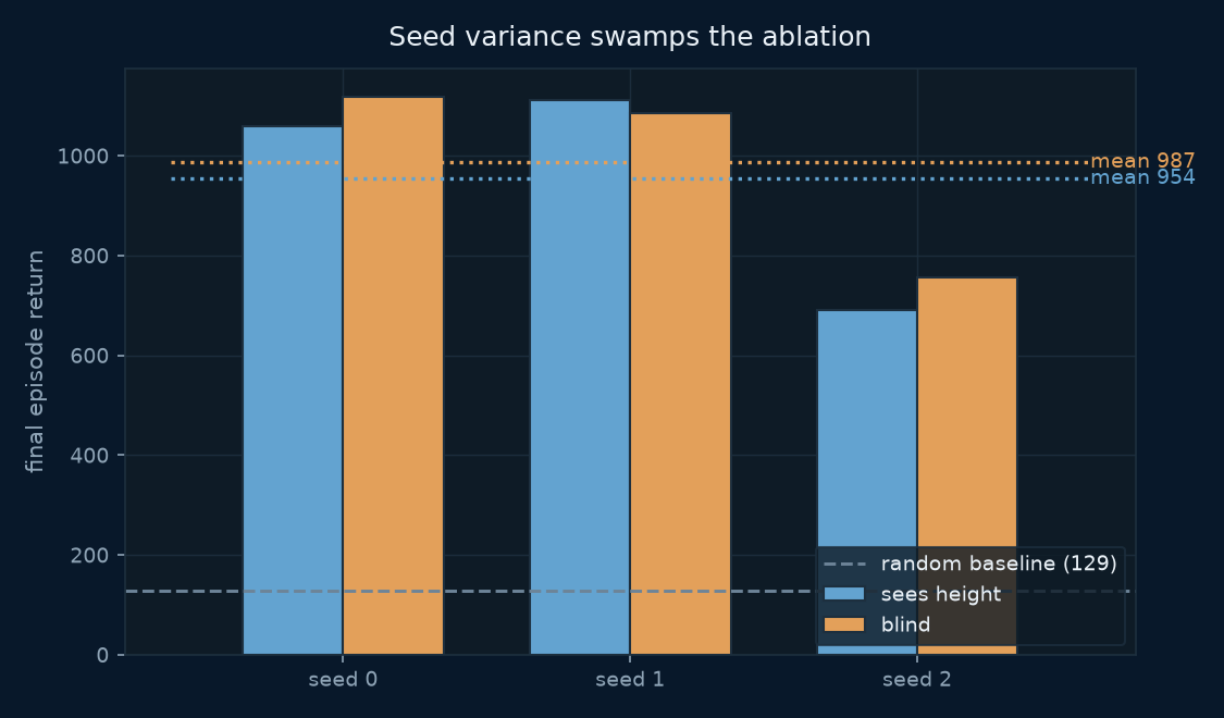
The blind policy scored marginally higher. The honest reading is not "blindness helps" — it is that the seed spread (692 to 1119) is an order of magnitude larger than the gap between arms, so there is no measurable effect.

One run per arm would have produced a confident wrong answer

And did, twice, in opposite directions, before the seeds were run. The first comparison showed the seeing policy ahead; the second showed the blind policy ahead by more. Both were single runs. Both were noise.

Why it failed, most likely

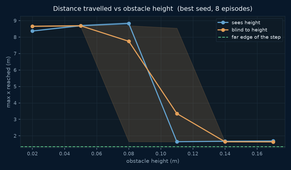
Both policies behave almost identically across the height range, and both fall off the same cliff between 0.08 m and 0.11 m. Below it they travel about 8 m. Above it they stop at 1.65 m — just past the step, and then nothing.

So the task does not appear to require perception. One robust hopping gait clears everything below the cliff, and nothing clears what is above it. If there is no behaviour worth adapting, seeing the height buys nothing.

That is a statement about this height range on this robot, not about obstacle perception in general. Widening the range until adaptation is forced is lab 2's business.

The bug that looked exactly like success

An earlier version of this lab trained to a 100% clear rate at every obstacle height. Every metric looked right.

Running the same policy with the obstacle removed entirely gave an identical distance, an identical episode length, and climbed was 0/8 throughout. The robot was diving forward and falling over at one second, and the box never impeded it at all.

The clear rate was real, reproducible, and measured nothing.

The check that catches it

test_the_obstacle_actually_obstructs tests the physics directly rather than through a policy: a robot resting over the box must sit higher than one on open floor, by the height of the box. Measured +0.049 m for a 0.05 m box and +0.099 m for a 0.10 m one.

It took three attempts to write. The first left the foot 0.15 m inside the box, so MuJoCo ejected the robot. The second lifted both placements, so they settled identically. The third ran for 250 steps — long enough for an unactuated robot to collapse under gravity in both arms, landing in a heap at the same height regardless of what was underneath it.

All three reported exactly 0.000. A test that keeps reporting zero is usually measuring its own setup.

Where DeepSpeed is, and is not

The policy is 10,119 parameters. ZeRO partitions optimizer state, gradients and parameters; all three are rounding errors at this size. There is nothing to shard.

Measured, rather than assumed:

configuration	CPU	CUDA (RTX 3080 Ti)	CPU faster by
4 envs (--dry-run)	682 steps/s	341 steps/s	2.0×
16 envs (the default)	2,513 steps/s	1,480 steps/s	1.7×

Median of repeated paired runs; CPU won 5 of 5 with no overlap between the two sets. Note the gap narrows as the environment count rises, which is the whole story — see below.

The policy is 10,119 parameters. The matrix multiplications are trivial; the cost is MuJoCo stepping environments, which happens on the CPU either way, so moving a 10k-parameter forward pass to a GPU adds a host-device transfer to the part that was never the bottleneck.

The ratio is scoped to the environment count, and that matters more than the ratio. At 4 environments the GPU is 2.0× behind; at 16 it is 1.7×. Extrapolating the trend rather than the number: with enough parallel environments the GPU should win, which is exactly why GPU-resident simulators exist. The useful conclusion is not "CPU is faster" but "the policy was never the bottleneck — parallelism in the SIMULATOR is the lever."

So --device auto resolves to CPU here. --device cuda is supported and reported, not recommended. This lab is the seventh declared launcher="python" exception.

That is not an apology for the category. It is the first rung.

This paragraph used to predict that "lab 2 is a 7B vision-language-action policy needing ~27 GB for LoRA". That never happened — lab 2 is another small-policy study (11,597 parameters) and lab 3 is a 193k-parameter vision student, which is the first place in this category a GPU wins at all (13.6×) and is still not a sharding problem. The direction is right and the timetable was invented; VLA models at 7B are genuine ZeRO territory, the same shape as gpt_oss_lora, and this course has not reached them. A page that predicts the future dates badly.

tests/test_obstacle_hopper.py fails if the policy ever exceeds 1M parameters, so that justification cannot go stale quietly.

What is exactly testable here

PPO's two components are pure tensor arithmetic, so they are checkable on a CPU with no simulator attached. GAE has two derived limits:

$$\begin{aligned} \lambda = 1 &\;\Rightarrow\; \text{discounted Monte-Carlo return} - V(s) \\[2pt] \lambda = 0 &\;\Rightarrow\; r + \gamma V(s') - V(s) \end{aligned}$$

An off-by-one in the backward recursion, a dropped (1 - done) mask, or a flipped sign all still produce plausible advantages and a run that trains to something. None of them survive those two limits, which the suite asserts to 1e-6 against independently computed references.

The clipped objective has one too: past the clip boundary, in the direction that would improve the objective, the gradient must be exactly zero. That is the entire trust region, and taking max instead of min leaves a loss that still descends with the constraint quietly removed.

Relation to the RLHF thread

03_llms/06_grpo is this algorithm with the critic deleted — in that setting rewards are sparse, verifiable and comparable within a group of samples for one prompt, so a learned value function earns nothing.

Here rewards are dense and shaped: forward velocity on every step. The critic has real work to do and stays. Same algorithm family, opposite call, for a stated reason.

Next step: how this scales to real humanoid work

The obvious guesses are more data, more GPU, a bigger network. For this kind of work the first two are mostly wrong and the third is almost always wrong, which is worth knowing before spending money on any of them.

Data is free and that is not the bottleneck. A simulator generates infinite fresh experience — this lab produced 600,000 transitions in eight minutes on a laptop. Reinforcement learning from scratch is not data-limited the way supervised learning is. It is limited by exploration: whether the policy ever stumbles into the behaviour you are paying it for. Doubling the steps on a task the robot cannot discover changes nothing, and the flat seed on the learning curve above is a 600,000-step run that learned to stand still.

The GPU story is real, but it is about the simulator, not the policy. Measured here: CPU beat an RTX 3080 Ti by 1.7–2.0× depending on the environment count, because a 10k-parameter network is not work. What is work is stepping physics for thousands of environments at once — and that is exactly what GPU-resident simulators exist for. MuJoCo Playground (pip install playground) runs MJX on-device and reports most of its environments training in under ten minutes on one GPU; Isaac Lab and Brax occupy the same niche. Moving from 16 CPU environments to thousands of GPU ones is the single biggest practical speed-up available, and it changes nothing about the algorithm.

So the honest ordering of what to change:

change	what it actually costs you	worth it when
Degrees of freedom	exploration difficulty, super-linearly	always — it is the real curriculum
GPU-parallel simulator	a rewrite into JAX (MJX/Brax) or Isaac	the moment one run takes more than an hour
Reward shaping	your afternoons	constantly; it is where most of the work is
Bigger policy	almost nothing, and it rarely helps	only once observations become pixels
More steps on the same task	time	only if the curve is still climbing

Degrees of freedom are the real difficulty axis

This robot has three actuated joints and a torso that cannot rotate. Gymnasium's Walker2d has six and can fall over; Humanoid has seventeen and must balance in three dimensions. Each step along that ladder is a large jump in how long a policy flails before it finds anything, because the space of things to try grows with every joint while the fraction of them that help shrinks.

Concretely, in increasing order of pain, and all of them runnable from what is already in this folder:

1. Un-comment the rooty hinge. One line. The torso can now tip, and you have a genuinely hard balance problem. Expect millions of steps and expect to need reward terms you have not thought of yet.
2. Swap the XML for Walker2d or Ant. Gymnasium ships the models; the training loop here does not care which robot it is driving.
3. Add obstacles, then randomise them. A second box, then varying spacing as well as height. This is domain randomisation, and the obstacle-height range in this lab is already a one-variable version of it.
4. Move to a GPU-parallel simulator once a run stops fitting in a coffee break.

Where data finally becomes the answer

Everything above is reinforcement learning from scratch, where the simulator is the data source and human effort goes into rewards. There is a second path, and it is where the field has moved for manipulation: learn from demonstrations instead of from reward.

That flips every constraint. Demonstrations are scarce and expensive — somebody teleoperates a real robot — so now data really is the bottleneck, and reward engineering largely disappears. LeRobot is the open ecosystem for it: a shared dataset format, pretrained policies, and simulated environments on the Hub.

And it is where the subject of this course finally bites. A vision-language-action model such as OpenVLA-7B needs roughly 27 GB for LoRA fine-tuning at minimum and 60–72 GB at a useful batch size. That does not fit on one consumer card, and it is the same ZeRO-plus-LoRA problem as gpt_oss_lora — a 7B policy instead of a 10k one.

That is the arc of this category: toy physics → more joints → parallel simulation → learned-from-demonstration policies that do not fit on one card. This page is the first rung, and the honest reason it needs no GPU is that the first rung does not.

Run it

Cold start to a trained robot, with nothing installed. The whole thing is CPU-only — no GPU, no model download, no graphics stack.

1. Get the repo and the toolchain

git clone https://github.com/yiqiao-yin/deepspeed-course.git
cd deepspeed-course/07_physical_ai/01_obstacle_hopper

Everything here uses uv. If you do not have it:

curl -LsSf https://astral.sh/uv/install.sh | sh

uv sync      # reads the committed uv.lock; ~1 min the first time

2. Look at the world before training anything

uv run obstacle_env.py

BASELINE, random policy, low  (walk over)  [0.02, 0.06] m
  mean return  130.58   mean max x  0.530 m   cleared 0/10
BASELINE, random policy, high (must climb)  [0.12, 0.17] m
  mean return  115.56   mean max x  0.475 m   cleared 0/10

cleared 0/10 is the point. A random policy never gets past the step, so there is something to learn. Run this before trusting any trained number.

3. Check the algorithm without a simulator

uv run ppo.py                               # the two GAE limits
uv run ../../tests/test_obstacle_hopper.py  # 28 property checks

lambda=1 matches Monte-Carlo minus baseline : max err 4.77e-07
lambda=0 matches the one-step TD residual   : max err 0.00e+00
policy+value parameters: 10,119
...
28/28 checks passed

Both run in seconds. If the second one fails, stop — the physics or the advantages are wrong and no amount of training will fix it.

4. Train

uv run train_ppo.py --dry-run     # 30 s: proves the pipeline assembles
uv run train_ppo.py               # the real run, ~8 min on CPU

Watch the cleared column. It sits at 0% for a long while — the robot is learning to stand before it can learn to travel — and then moves sharply. Expect something like:

  565,248 steps  return   986.7  max_x  4.30m  cleared  100%  (low 100% / high 100%)   438s

against the baseline's return 129, cleared 0%. If it is still at 0% after 600k steps, that is a legitimate outcome, not a broken install — one of the three seeds on the chart above never breaks through either. Re-run with --seed 1.

5. The ablation, and the figures

uv run train_ppo.py --total-steps 600000 --seed 0 --name seeing_s0
uv run train_ppo.py --total-steps 600000 --seed 0 --name blind_s0 --blind-to-height
uv run make_figures.py

make_figures.py needs both arms for the comparison plots, and tells you which run is missing if you only have one. For the seed-spread chart on this page, repeat with --seed 1 and --seed 2; six runs is about forty-five minutes, or eight if you run them in parallel — they are independent processes.

6. Pictures of the robot (optional)

uv run render.py            # the world stills and both HUD animations

This is the only part that needs OpenGL, and it is deliberately separate: training uses state observations and never opens a graphics context. If no backend is available the script says so and exits cleanly rather than breaking anything else. It probes glfw, egl and osmesa in that order and reports which one worked.

What you end up with

runs/<name>/curve.csv      every evaluation during training
runs/<name>/summary.json   baseline, final scores, wall time, device
runs/<name>/policy.pt      the trained weights + observation normaliser

Every figure on this page is generated from those files, so nothing here can show a result a run did not produce.

References

• Schulman et al., Proximal Policy Optimization, 2017
• Schulman et al., Generalized Advantage Estimation, 2015
• MuJoCo · Gymnasium
• Kim et al., OpenVLA, 2024 — where this category is heading