RL for Trading

Reading this without a background in machine learning

The plain words boxes carry the whole story; the technical detail around them is there if you want it.

The one line version: a model that guesses tomorrow's market direction better than a coin flip still loses money once you pay trading fees. Training the same network to chase money instead of accuracy does not beat simply buying and holding either — but it loses far less when the market crashes, and that turns out to be the only thing reinforcement learning buys here.

Baseline: buy and hold all nine sectors — 13.7%/yr, Sharpe 0.79, worst drawdown −36.9% — plus RSP, the equal-weight S&P 500 index, at 12.9%. Any method that cannot beat doing nothing clever has not earned its compute. Budget: 120 PPO/GRPO iterations over 2,992 training days, three seeds per arm, 5 bps per side. Train 2004–2015, test 2016–2025, nothing shuffled.

Falsifier A: the reward-driven arms must cut the worst drawdown by a third against buy-and-hold while keeping 70% of its return. Falsifier B: GRPO's dollar-neutral book must be positive, or the group baseline did not learn to pick sectors and any gain is market timing in a long-short costume.

A supervised model predicts tomorrow's return at 51.1% directional accuracy — genuinely better than chance — and trading it loses 2.2% a year. The same network, same features, optimised on money after costs instead of squared error, cuts the worst drawdown nearly in half and makes +6.1% through the COVID crash while the market loses 28.8%.

This is the matched pair to 02_rnn_stock_data: one predicts, the other decides.

Result

arm	ann	95% CI	Sharpe	maxDD	turnover	params
buyhold	13.7%	—	0.79	−36.9%	0.000	—
rsp_index	12.9%	—	0.69	−39.0%	—	—
ppo	9.8%	[+3.0, +16.8]	0.72	−20.6%	0.092	9,731
grpo	10.4%	[+2.3, +18.1]	0.69	−24.9%	0.071	4,866
grpo_neutral	−1.5%	[−2.9, −0.2]	−0.61	−15.5%	0.086	4,866
forecast_band	−1.2%	[−6.8, +3.9]	−0.10	−32.2%	0.430	—
forecast_rule	−2.2%	[−8.6, +3.9]	−0.18	−40.8%	0.557	—
flat	0.0%	—	0.00	0.0%	0.000	—
random	−17.2%	[−21.7, −13.0]	−2.42	−82.1%	1.012	—

2,428 held-out days, median of three seeds, spread published below. Intervals are a stationary block bootstrap over 21-day blocks — a t-test on daily returns pretends 2,428 observations are independent and finds significant edges in pure noise.

Per seed, because a median hides the spread:

arm
ppo	+9.4%	+9.8%	+10.5%
grpo	+9.9%	+10.4%	+12.1%
grpo_neutral	−2.4%	−1.5%	−1.0%

In plain words. Guessing tomorrow's price slightly better than a coin flip does not make money — after trading fees it loses. Training the same network to maximise money instead of accuracy does not make more money than simply buying and holding either, but it loses a lot less when the market crashes.

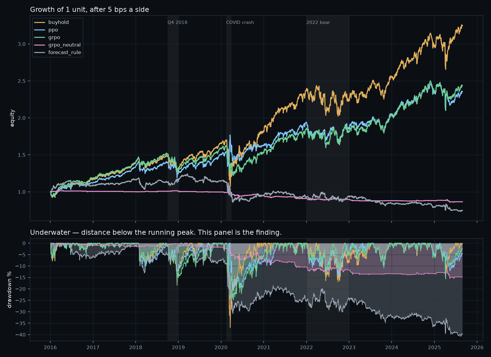
By regime

The lower panel of that figure is the finding. In numbers, cumulative over each drawdown:

arm	Q4 2018 (63d)	COVID (31d)	2022 bear (251d)	the other 2,083 days, ann
buyhold	−12.7%	−28.8%	−6.1%	21.7%
rsp_index	−13.9%	−31.8%	−11.8%	22.1%
ppo	−11.2%	+6.1%	−4.2%	12.3%
grpo	−13.3%	−16.3%	−2.2%	15.7%
forecast_rule	+2.7%	−12.0%	+0.6%	−1.9%

PPO made +6.1% through the COVID crash while the market lost 28.8%, and it pays for that with 12.3% against 21.7% across the calm 86% of the sample. That is the whole trade, and it is not free.

In plain words. The trained policies are insurance, not a money machine. They give up about a third of the good years to lose much less in the bad weeks. Whether that is a good deal depends on what you are trying to do.

The falsifiers

A. Risk — split.

	drawdown cut	return kept
ppo	44%	72%	HOLDS
grpo	32.5%	76%	FAILS

The bar was a third, written down before any arm was trained. GRPO lands at 32.5% — short by 0.8 of a point. The bar has not been moved.

B. Selection — fails, and it was my hypothesis.

GRPO scores each sample against its group mean. Here the group is every sector on one day, so the baseline is the equal-weight market return and the advantage is an excess return. The prediction was that long-short equity would fall out of the algorithm for free.

It does not. Strip out the net market exposure and the dollar-neutral book returns −1.5%/yr, 95% CI [−2.9%, −0.2%] — entirely below zero. The group baseline did not learn which sector beats which. The gain in the table above is market timing wearing a long-short costume, and the lab says so.

What survives is narrower and real: GRPO matches PPO on every measure with half the parameters, because it carries no critic. The baseline it does not have to learn is exactly the one a critic spends 4,865 parameters estimating.

Problem setup

Universe	all nine SPDR sector ETFs — XLB, XLE, XLF, XLI, XLK, XLP, XLU, XLV, XLY
Action	a target weight in [−1, +1] per sector, per day
State	8 features for that sector today plus the position currently held in it
Reward	`w · r_next − cost ·
Cost	5 bps per side, charged on the change in position
Train / test	2,992 days to 2015-12-31 / 2,428 days from 2016-01-04
Features	1/5/20-day returns, 20-day volatility, distance from the 14/50/200-day moving averages, RSI-14

The reward is the P&L. No shaping, no auxiliary prediction loss, no risk penalty. Everything here is what falls out of optimising money after costs, which is the only way the comparison against a squared-error forecast means anything.

Why the position is in the state

Three things decide whether a forecast is worth acting on, and a loss on tomorrow's price cannot express any of them:

$$\text{pnl}_{i,t} \;=\; \underbrace{w_{i,t}\, r_{i,t}}_{\text{the call}} \;-\; \underbrace{c\,\lvert w_{i,t} - w_{i,t-1}\rvert}_{\text{the act}}$$

Holding is free and flipping is not, so being long and going long are different acts. A correct forecast with a small edge is unprofitable. And the objective is a path: market.py shuffles one return series 400 ways and gets an identical +18.3% annualised in every ordering with worst drawdowns ranging −23.3% to −71.2% — a 48-point spread the mean cannot see.

The two methods, and the one line between them

PPO and GRPO share the network, the clipped surrogate, the data and the budget. They differ only in where the advantage baseline comes from, which is why they live in one file — the 03_llms/05_dpo precedent.

PPO fits a critic and bootstraps:

$$\hat A_t \;=\; \sum_{l\ge 0}(\gamma\lambda)^l \delta_{t+l}, \qquad \delta_t = r_t + \gamma V(s_{t+1}) - V(s_t)$$

GRPO has no critic. Each sample is scored against the mean of its group, and here the group is every sector on the same day:

$$\hat A_{i,t} \;=\; \frac{r_{i,t} - \frac{1}{N}\sum_{j} r_{j,t}} {\operatorname{std}_j\!\left(r_{j,t}\right)}$$

The numerator is the excess return over an equal-weighted market. The baseline is not approximated by a network — it is the market, exactly, for free, every day. Both arms then maximise the same clipped surrogate:

$$L^{\text{CLIP}}(\theta) = \hat{\mathbb{E}}\!\left[\min\!\left( \rho\hat A,\; \operatorname{clip}(\rho, 1-\epsilon, 1+\epsilon)\hat A \right)\right], \qquad \rho = \frac{\pi_\theta(a\mid s)}{\pi_{\theta_{\text{old}}}(a\mid s)}$$

Survivorship bias, measured rather than waved at

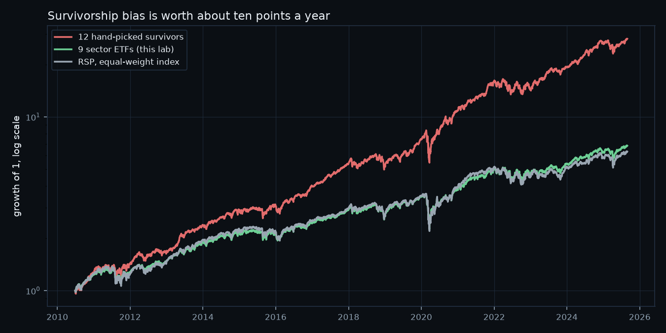
The obvious universe for a trading lab is a handful of well-known stocks. That universe is poisoned, and this lab measured it before choosing anything:

universe	2010–2025, equal weighted	vs RSP
12 hand-picked large caps, liquid today	+23.70%	+9.91%
9 sector ETFs (what this lab uses)	+14.08%	+0.28%
RSP, S&P 500 equal weight	+13.80%	—

Choosing in 2026 twelve companies that happened to survive is worth ten points a year. Buy-and-hold is the control every RL arm must beat, so on that basket the control gets a ten-point head start it did not earn and RL "loses" for reasons that have nothing to do with RL.

Sector ETFs do not have the problem: when a constituent fails or is acquired, the ETF absorbs it internally and the price already reflects it. And there is no basket to pick — the lab takes all nine, so there is no selection decision to be biased by.

The textbook fix is unavailable here, and the page says so. Sixteen delisted tickers were tested against yfinance — SIVB, FRC, Twitter, Activision, Monsanto, Raytheon — and fourteen return nothing at all. The two that appear to work are traps: SBNY returns 261 rows beginning in 2024, a different company recycling a dead ticker. The bias is routed around and bounded, not designed away.

Reproduce with uv run data.py --bias.

Where DeepSpeed earns its place, and where it does not

The honest answer for every arm above is nowhere. GRPO is 4,866 parameters and PPO 9,731 — 0.08 and 0.16 MB of weights, gradients and Adam state. Sharding 0.08 MB across eight cards saves 0.01 MB a card and costs an all-gather every step, so train_rl.py runs plain python by default.

The real bottleneck is not memory: the rollout is sequential over 2,992 days, because the position on day t depends on the action on day t−1. That does not shard at all.

Scale to a cross-sectional model over 500 stocks and it becomes a real question — and the answer is the one 06_protein_folding reaches from a completely different direction:

rung	params	wt+Adam	activations	ratio	ZeRO-3 total saving
xl, 500 assets, d=1024	151M	2.4 GB → 0.3	14.7 GB	6.1×	12%
xxl, 500 assets, d=2048	805M	12.9 GB → 1.6	39.3 GB	3.1×	22%

Activations dominate and ZeRO does not shard activations. Every rank pays them in full. An Evoformer trunk is ~100k parameters, fills a card with O(N²) pair representations, and shows ZeRO-1 against ZeRO-3 differing by 4.6%. Two unrelated domains, one systems fact: shard the thing that is actually large, and when that is the activations the tool is gradient checkpointing.

uv run capacity.py --measure builds each rung on the meta device and confirms the arithmetic to within 1.2%.

Where the edge dies

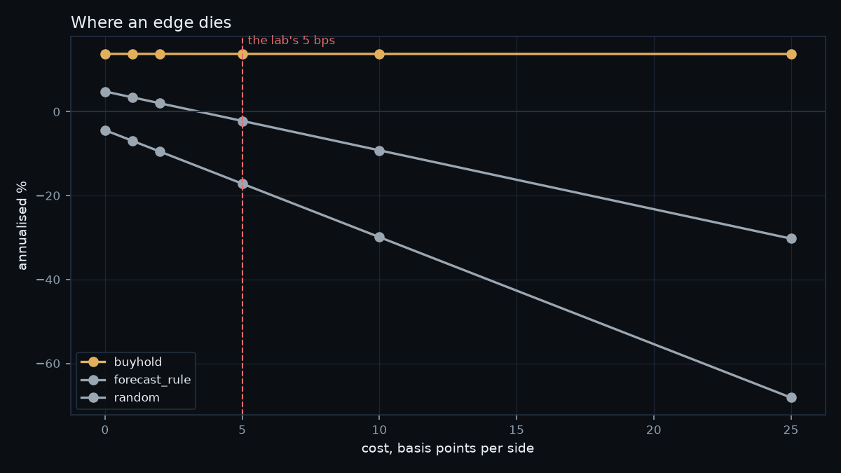
book	0 bps	5 bps	25 bps
always long	13.8%	13.7%	13.7%
perfect foresight	228.2%	215.5%	164.8%
coin flip, daily	−4.4%	−17.2%	−68.2%

Perfect foresight survives any cost; a coin flip is destroyed by the smallest. A method that only wins at 0 bps has not been shown to win, which is why no number on this page is quoted without its cost.

Prior work — the algorithms here are not ours

Neither method originates in this lab, and reinforcement learning for trading is a large and old literature. What is assembled here is the comparison and its controls.

Schulman, Wolski, Dhariwal, Radford & Klimov (2017), Proximal Policy Optimization Algorithms · arXiv:1707.06347	The clipped surrogate every arm optimises.
Schulman, Moritz, Levine, Jordan & Abbeel (2015), High-Dimensional Continuous Control Using Generalized Advantage Estimation · arXiv:1506.02438	GAE($\lambda$), which supplies PPO's advantage here.
Shao et al. (2024), DeepSeekMath: Pushing the Limits of Mathematical Reasoning in Open Language Models · arXiv:2402.03300	GRPO. The group-relative baseline that replaces the critic. Introduced for language models, where a group is several sampled answers to one prompt; this lab's only move is to make the group every sector on the same day, which turns the baseline into the equal-weight market return.
Moody & Saffell (2001), Learning to Trade via Direct Reinforcement, IEEE Trans. Neural Networks 12(4)	The original argument that a trading policy should optimise a financial objective directly rather than forecast and then act, including transaction costs and the position as state. This lab's premise is theirs, restated.
Deng, Bao, Kong, Ren & Dai (2017), Deep Direct Reinforcement Learning for Financial Signal Representation and Trading, IEEE Trans. Neural Networks and Learning Systems 28(3)	The deep-network successor to Moody & Saffell.
Politis & Romano (1994), The Stationary Bootstrap, JASA 89(428)	The block bootstrap behind every confidence interval on this page.

What this lab adds, scoped honestly

A survivorship-bias control with a number attached. Most RL-for-trading results are reported on a basket of names that exist today. Measured here, that choice is worth +9.91%/yr against an unbiased index — larger than any effect in the table above, and it accrues to buy-and-hold, the control every RL arm must beat. uv run data.py --bias reproduces it.

A dollar-neutral arm that refutes the obvious story about GRPO. The group baseline looks like it should produce long-short selection for free. Strip the market exposure out and the book returns −1.5%/yr, CI [−2.9%, −0.2%]. The gain is market timing. We know of no paper making that specific negative claim, and we are not confident none exists.

Neither is a paper. The method is Schulman's and Shao's; the premise is Moody and Saffell's; this page is for watching all of it fail to beat buy-and-hold on a dataset you can re-run in two minutes.

Limitations

One market, one decade, three seeds. The test window is 2016–2025 US equities. The GFC sits in the training window, so the largest drawdown in the data never tests the claim. Three seeds is the minimum and still thin — the per-seed spread on grpo is 2.2 points against an effect of 3.9.

The headline is a risk claim, not a return claim. Both reward-driven arms lose to buy-and-hold on return. Anyone reading this as a trading strategy has read it wrong.

Free, retail-grade data. Yahoo adjusted closes, prices only — no volume, no fundamentals, no intraday, no order book, no borrow cost for the short side. The dollar-neutral arm in particular assumes shorting is free, which it is not.

The costs are a guess. 5 bps per side is plausible for a liquid ETF and is not a measurement. The cost curve is published so you can find your own.

Environment & Local Testing

cd 02_intermediate/05_rl_trading
uv sync

uv run data.py                # the frozen panel, and the drawdowns in it
uv run data.py --bias         # what picking survivors is worth
uv run data.py --leakage      # prove no feature reads forward
uv run market.py --cost-curve # the arithmetic, and where an edge dies
uv run capacity.py            # the ladder and what ZeRO can shard
uv run baselines.py           # everything the learned arms must beat

All of the above are CPU-only, need no network, and finish in seconds to a minute. The data is committed — 659 KB of adjusted closes — because vendor history is not immutable and a course that pins numbers to a live feed is publishing figures nobody can check. uv run data.py --refresh re-downloads deliberately and prints what moved.

Reproduce the arms:

./run_arms.sh                 # 9 runs, ~2 min each on CPU
uv run evaluate.py --json results.json
uv run render_figs.py

Runs end to end on one machine	Yes
GPU required	No — and capacity.py explains why
Downloads	none; the panel is committed

CoreWeave

sbatch run_deepspeed.sh
squeue -u $USER
tail -f logs/rl_trading_*.out

RunPod

uv run ../../runpod/runpod_ctl.py run 02_intermediate/05_rl_trading \
    --dry-run --collect --wait --terminate --yes
uv run ../../runpod/runpod_ctl.py pods

Files

file	role
data.py	the frozen panel, the bias report, the look-ahead check
market.py	positions, costs, P&L, and assert_causal
baselines.py	buy-and-hold, RSP, flat, random, forecast, forecast+band
train_rl.py	the entry point — --method ppo|grpo
evaluate.py	regime split, block bootstrap, the falsifiers
capacity.py	the cross-sectional ladder and the ZeRO table
render_figs.py	equity, drawdown, cost curve, bias
data/sectors.csv	659 KB, 2003–2025, committed
data/survivors.csv	491 KB, the deliberately biased basket

Logic test: tests/test_rl_trading.py — 24 checks, no GPU, no network.

See also

02_intermediate/02_rnn_stock_data is the other half of this pair. It predicts avg_delta with an RNN and scores itself with Theil's U against a persistence baseline and directional accuracy against a coin flip — the right discipline for a forecast. This lab takes the same data and asks what a forecast is worth once you have to act on it.